Detailed Example#

Compared to the simple example, in this detailed example, we will also determine the explicit form of the mass matrices for the flavor model introduced in “Are neutrino masses modular forms?” by F. Feruglio (https://arxiv.org/pdf/1706.08749) as so-called Example 1 in section 3.12. The chiral supermultiplets and their transformation properties of this model are

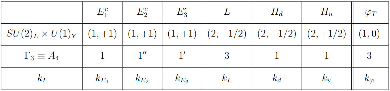
../_images/simpleexample_constructterms_table.png

where \(k_L=1\), \(k_u=0\), \(k_\varphi=-3\), and \(k_{E_i}+k_L+k_d+k_\varphi=0\). Table taken from https://arxiv.org/pdf/1706.08749.

Import#

# Import the constructterms module of FlavorPy
import flavorpy.constructterms as ct

Define Groups#

Analogous to the simple example, we start by defining the non-Abelian group \(A_4\). Only this time, we also define specific clebsch-gordan coefficients

# Representations of A4
A4_reps = ['1', '1p', '1pp', '3']

# Tensor products of A_reps as a matrix, i.e. A_tensor_procuts[i,j,] = A4_reps[i] x A4_reps[j]
A4_tensor_products = [[['1'], ['1p'], ['1pp'], ['3']],
                      [['1p'], ['1pp'], ['1'], ['3']],
                      [['1pp'], ['1'], ['1p'], ['3']],
                      [['3'], ['3'], ['3'], ['1', '1p', '1pp', '3', '3']]]

# To determine the components of the mass matrix, we need to define the clebsch gordans for a specific basis.
# In this case we will use the so-called "complex basis" specified in Appendix C of the paper
A4_clebsches = {'1 x 1': {'1': [[[1]]]},
                '1 x 1p': {'1p': [[[1]]]},
                '1 x 1pp': {'1pp': [[[1]]]},
                '1p x 1p': {'1pp': [[[1]]]},
                '1p x 1pp': {'1': [[[1]]]},
                '1pp x 1pp': {'1p': [[[1]]]},
                '1 x 3': {'3': [[[1,0,0],[0,1,0],[0,0,1]]]},
                '1p x 3': {'3': [[[0,0,1],[1,0,0],[0,1,0]]]},
                '1pp x 3': {'3': [[[0,1,0],[0,0,1],[1,0,0]]]},
                '3 x 3': {'1': [[[1,0,0, 0,0,1, 0,1,0]]],
                          '1p': [[[0,1,0, 1,0,0, 0,0,1]]],
                          '1pp': [[[0,0,1, 0,1,0, 1,0,0]]],
                          '3': [[[" 2/sqrt(3)",0,0, 0,0,"- 1/sqrt(3)", 0,"- 1/sqrt(3)",0],
                                 [0,"- 1/sqrt(3)",0, "- 1/sqrt(3)",0,0, 0,0," 2/sqrt(3)"],
                                 [0,0,"- 1/sqrt(3)", 0," 2/sqrt(3)",0, "- 1/sqrt(3)",0,0]],
                                [[0,0,0, 0,0,1, 0,-1,0],
                                 [0,1,0, -1,0,0, 0,0,0],
                                 [0,0,-1, 0,0,0, 1,0,0]]]}}

# Construct A4 Group
A4 = ct.NonAbelianGroup('A4', representations=A4_reps,
                        tensor_products=A4_tensor_products, clebsches=A4_clebsches)

# Construct Modular Weight "group"
mod_weight = ct.U1Group('mod weight')

# Construct U(1) Hypercharge
U1y = ct.U1Group('U1y')

Define Fields#

Next, we can define the fields of the flavor model. Compared to the simple example we now also give explicit components under the A4 symmetry.

It is very important to note that ConstructTerms can only handle one non-Abelian group or multiple non-Abelian groups that commute with each other, i.e. a direct product of multiple non-Abelian groups. Do not assign charges of two separate non-Abelian groups, if they do not commute!

ke = 20
kd = - ke + 1 - 3

E1 = ct.Field('E1', charges={A4:['1'], mod_weight:ke, U1y:1}, components={A4: {'1': [['e1']]}})
E2 = ct.Field('E2', charges={A4:['1pp'], mod_weight:ke, U1y:1}, components={A4: {'1pp': [['e2']]}})
E3 = ct.Field('E3', charges={A4:['1p'], mod_weight:ke, U1y:1}, components={A4: {'1p': [['e3']]}})
L = ct.Field('L', charges={A4:['3'], mod_weight:-1, U1y:-1/2}, components={A4: {'3': [['l1', 'l2', 'l3']]}})
Hd = ct.Field('Hd', charges={A4:['1'], mod_weight:kd, U1y:-1/2}, components={A4: {'1': [['hd']]}})
Hu = ct.Field('Hu', charges={A4:['1'], mod_weight:0, U1y:+1/2}, components={A4: {'1': [['hu']]}})
PhiT = ct.Field('PhiT', charges={A4:['3'], mod_weight:3, U1y:0}, components={A4: {'3': [['phi1', 'phi2', 'phi3']]}})
Y = ct.Field('Y', charges={A4:['3'], mod_weight:2, U1y:0}, components={A4: {'3': [['y1', 'y2', 'y3']]}})

all_fields = [E1, E2, E3, L, Hd, Hu, PhiT, Y]

W = ct.Field('W', charges={A4:['1'], mod_weight:0, U1y:0})

As a side remark, it is also possible to determine the product of two fields, which again yields an instance of the Field class, i.e.

LxPhiT = L.times(PhiT)
print('LxPhiT.charges: ', LxPhiT.charges, '\n')
print('LxPhiT.components:', LxPhiT.components)

LxPhiT.charges:  {A4: ['1', '1p', '1pp', '3', '3'], mod weight: 2, U1y: -0.5}

LxPhiT.components: {A4: {'1': [['l1 phi1 + l2 phi3 + l3 phi2']], '1p': [['l1 phi2 + l2 phi1 + l3 phi3']], '1pp': [['l1 phi3 + l2 phi2 + l3 phi1']], '3': [['2/sqrt(3) l1 phi1  - 1/sqrt(3) l2 phi3  - 1/sqrt(3) l3 phi2', '- 1/sqrt(3) l1 phi2  - 1/sqrt(3) l2 phi1 +  2/sqrt(3) l3 phi3', '- 1/sqrt(3) l1 phi3 +  2/sqrt(3) l2 phi2  - 1/sqrt(3) l3 phi1'], ['l2 phi3 - l3 phi2', 'l1 phi2 - l2 phi1', '- l1 phi3 + l3 phi1']]}}

Determine symmetry invariant terms in the superpotential#

Then we can determine the symmetry invariant terms up to a specific order of the superpotential with

allowed_products = ct.list_allowed_terms(all_fields, W, order=5)
allowed_products

[L L Hu Hu Y, E1 L Hd PhiT, E2 L Hd PhiT, E3 L Hd PhiT]

Moreover to obtain the explicit components of a term and determine the mass matrix call

product0 = allowed_products[0]
triv_A4_components = product0.components[A4]['1']
for term in triv_A4_components:
    print(term, "\n")

['(hu (hu (2/sqrt(3) l1 l1  - 1/sqrt(3) l2 l3  - 1/sqrt(3) l3 l2))) y1 + (hu (hu (- 1/sqrt(3) l1 l2  - 1/sqrt(3) l2 l1 +  2/sqrt(3) l3 l3))) y3 + (hu (hu (- 1/sqrt(3) l1 l3 +  2/sqrt(3) l2 l2  - 1/sqrt(3) l3 l1))) y2']

['(hu (hu (l2 l3 - l3 l2))) y1 + (hu (hu (l1 l2 - l2 l1))) y3 + (hu (hu (- l1 l3 + l3 l1))) y2']

Here the first term of the product L L Hu Hu Y yields the mass matrix

\[\begin{split}M_\nu ~=~ \dfrac{hu\,hu}{\sqrt{3}} ~\begin{pmatrix} 2\,y1 & -y3 & -y2 \\ -y3 & 2\,y2 & -y1 \\ -y2 & -y1 & 2\,y3 \end{pmatrix},\end{split}\]

while the second term yields

\[\begin{split}\tilde M_\nu ~=~ hu\,hu ~\begin{pmatrix} 0 & y3 & -y2 \\ -y3 & 0 & y1 \\ y2 & -y1 & 0 \end{pmatrix},\end{split}\]

which is antisymmetric and hence does not contribute to the neutrion mass. In total we can obtain the same mass matrix as the paper, see eq. (38).

For the products that give mass to the charged leptons we get

products13 = allowed_products[1:]
triv_A4_components = [product.components[A4]['1'] for product in products13]
for term in triv_A4_components:
    print(term, "\n")

[['hd e1 l1 phi1 + hd e1 l2 phi3 + hd e1 l3 phi2']]

[['hd e2 l2 phi1 + hd e2 l3 phi3 + hd e2 l1 phi2']]

[['hd e3 l3 phi1 + hd e3 l1 phi3 + hd e3 l2 phi2']]

Given that the second and third components of the flavon field PhiT vanish, i.e. phi2=phi3=0, the charged lepton mass matrix is diagonal and reads

\[\begin{split}M_e ~=~ hd\,phi1 ~\begin{pmatrix} \alpha & 0 & 0 \\ 0 & \beta & 0 \\ 0 & 0 & \gamma \end{pmatrix},\end{split}\]

where \(\alpha\), \(\beta\), \(\gamma\) are the symmetry invariant coupling coefficients in front of the three individual terms. This is in agreement with the result from the paper, see eq. (36)