The Weinberg Operator Model of arXiv:2006.03058

This example is based on the paper “Double Cover of Modular S4 for Flavour Model Building” from P. P. Novichkov, J. T. Penedo, and S. T. Petcov available under https://arxiv.org/pdf/2006.03058. We will study their Weinberg Operator Model introduced in section 6.1 of the paper and try to reproduce their model fitting results.

Import

# Import the modelfitting module of FlavorPy
import flavorpy.modelfitting as mf

# We will also need numpy and pandas
import numpy as np
import pandas as pd
pd.set_option('display.max_columns', None)  # This pandas setting allows us to see all columns
import cmath

Mass matrices

First we need to define a lot of modular forms. See eqs. (3.3), (3.14), and (3.15) in the paper.

### Weight 1/2 modular forms
def theta(tau):
    q = cmath.exp(2j*cmath.pi*tau/4)
    return 1 + 2*q**4 + 2*q**16
def eps(tau):
    q = cmath.exp(2j*cmath.pi*tau/4)
    return 2*q + 2*q**9 + 2*q**25

### Weight 3 modular forms
# Weight 3, rep 1hatprime
def Y31hp1(tau):
    return cmath.sqrt(3) * (eps(tau) * theta(tau)**5 - eps(tau)**5 * theta(tau))
# Weight 3, rep 3hat
def Y33h1(tau):
    return eps(tau)**5 * theta(tau) + eps(tau) * theta(tau)**5
def Y33h2(tau):
    return 1/2/cmath.sqrt(2) * (5 * eps(tau)**2 * theta(tau)**4 - eps(tau)**6)
def Y33h3(tau):
    return 1/2/cmath.sqrt(2) * (theta(tau)**6 - 5 * eps(tau)**4 * theta(tau)**2)
# Weight 3, rep 3hatprime
def Y33hp1(tau):
    return 1/2 * (-4 * cmath.sqrt(2) * eps(tau)**3 * theta(tau)**3)
def Y33hp2(tau):
    return 1/2 * (theta(tau)**6 + 3 * eps(tau)**4 * theta(tau)**2)
def Y33hp3(tau):
    return 1/2 * (-3 * eps(tau)**2 * theta(tau)**4 - eps(tau)**6)

### Weight 4 modular forms
# Weight 4, rep 1
def Y411(tau):
    return 1/2/cmath.sqrt(3) * (theta(tau)**8 + 14 * eps(tau)**4 * theta(tau)**4 + eps(tau)**8)
# Weight 4, rep 2
def Y421(tau):
    return 1/4 * (theta(tau)**8 - 10 * eps(tau)**4 * theta(tau)**4 + eps(tau)**8)
def Y422(tau):
    return cmath.sqrt(3) * (eps(tau)**2 * theta(tau)**6 + eps(tau)**6 * theta(tau)**2)
# Weight 4, rep 3
def Y431(tau):
    return 3/2 * (eps(tau)**2 * theta(tau)**6 - eps(tau)**6 * theta(tau)**2)
def Y432(tau):
    return 3/2/cmath.sqrt(2) * (eps(tau)**3 * theta(tau)**5 - eps(tau)**7 * theta(tau))
def Y433(tau):
    return 3/2/cmath.sqrt(2) * (-eps(tau) * theta(tau)**7 + eps(tau)**5 * theta(tau)**3)

Then we can define the mass matrices. See eqs. (6.5), (6.6) or (6.7), (6.8) or Appendix E of the paper.

def Me(params):
    tau = params['Retau'] + 1j * params['Imtau']
    Y31hp1x = Y31hp1(tau)
    Y33h1x = Y33h1(tau)
    Y33h2x = Y33h2(tau)
    Y33h3x = Y33h3(tau)
    Y33hp1x = Y33hp1(tau)
    Y33hp2x = Y33hp2(tau)
    Y33hp3x = Y33hp3(tau)
    return np.transpose((1/cmath.sqrt(3) * np.array([[Y31hp1x, 0, 0],
                                                     [0, 0, Y31hp1x],
                                                     [0, Y31hp1x, 0]], dtype=complex)
                         + params['a2t']/cmath.sqrt(6) * np.array([[0, -Y33hp2x, Y33hp3x],
                                                                   [-Y33hp2x, -Y33hp1x, 0],
                                                                   [Y33hp3x, 0, Y33hp1x]], dtype=complex)
                         + params['a3t']/cmath.sqrt(6) * np.array([[0, Y33h3x, -Y33h2x],
                                                                   [-Y33h3x, 0, Y33h1x],
                                                                   [Y33h2x, -Y33h1x, 0]], dtype=complex)
                        ))

def Mn(params):
    tau = params['Retau'] + 1j * params['Imtau']
    Y411x = Y411(tau)
    Y421x = Y421(tau)
    Y422x = Y422(tau)
    Y431x = Y431(tau)
    Y432x = Y432(tau)
    Y433x = Y433(tau)
    return params['n_scale']*(1/cmath.sqrt(3) * np.array([[Y411x, 0, 0],
                                                          [0, 0, Y411x],
                                                          [0, Y411x, 0]], dtype=complex)
                             - params['g2t']/2/cmath.sqrt(3) * np.array([[2 * Y421x, 0, 0],
                                                                         [0, cmath.sqrt(3) * Y422x, -Y421x],
                                                                         [0, -Y421x, cmath.sqrt(3)*Y422x]], dtype=complex)
                             + params['g3t']/cmath.sqrt(6) * np.array([[0, -Y432x, Y433x],
                                                                       [-Y432x, -Y431x, 0],
                                                                       [Y433x, 0, Y431x]], dtype=complex)
                             )

Parameter space

# Sampling functions
def lin_sampling(low=0, high=1):
    def fct():
        return np.random.uniform(low=low, high=high)
    return fct
def const_sampling(value=0):
    def fct():
        return value
    return fct

# Constructing the parameter space
ParamSpace = mf.ParameterSpace()
ParamSpace.add_dim(name='Retau', sample_fct=lin_sampling(low=-0.5, high=0.5), min=-0.5, max=0.5)
ParamSpace.add_dim(name='Imtau', sample_fct=lin_sampling(low=0.866, high=2), min=0.866, max=3.5)
ParamSpace.add_dim(name='a2t', sample_fct=lin_sampling(low=-10, high=10), min=-10, max=10)
ParamSpace.add_dim(name='a3t', sample_fct=lin_sampling(low=-10, high=10), min=-10, max=10)
ParamSpace.add_dim(name='g2t', sample_fct=lin_sampling(low=-10, high=10), min=-10, max=10)
ParamSpace.add_dim(name='g3t', sample_fct=lin_sampling(low=-10, high=10), min=-10, max=10)
ParamSpace.add_dim(name='n_scale', sample_fct=const_sampling(1.), vary=False)

Experimental data

Although the paper uses the experimental data of https://arxiv.org/pdf/2003.08511, we will use the recent results of NuFit v5.3 (see http://www.nu-fit.org/?q=node/278) in the following

ExperimentalData_NO = mf.NuFit53_NO
ExperimentalData_IO = mf.NuFit53_IO

Model construction

Since the paper does not consider the experimental data on the CPV angle ‘d/pi’ when fitting the model, we will also omit it here

MyModel_NO = mf.FlavorModel(name='MyModel_NO',
                            mass_matrix_e=Me,
                            mass_matrix_n=Mn,
                            parameterspace=ParamSpace,
                            ordering='NO',
                            experimental_data=ExperimentalData_NO,
                            fitted_observables=['me/mu','mu/mt','s12^2', 's13^2', 's23^2', 'm21^2', 'm3l^2'])

MyModel_IO = MyModel_NO.copy()
MyModel_IO.ordering = 'IO'
MyModel_IO.name = 'MyModel_IO'
MyModel_IO.experimental_data = ExperimentalData_IO

Fitting

Let us now scan the parameter space to find some viable points in the parameter space that yield observables, which are in agreement with the experimental data.

Normal Ordering

Fitting around 100 random points, which takes about 5 minutes, seems sufficient to find a lot of minima with \(\chi^2<1\)

# Running the fit. Takes about 5 minutes.
# Don't worry about warnings that might pop up when running this command. Only valid points will be further processed.
df_NO = MyModel_NO.make_fit(points=100)
df_NO.head(5)

	chisq	chisq_dimless	Retau	Imtau	a2t	a3t	g2t	g3t	n_scale	me/mu	mu/mt	s12^2	s13^2	s23^2	d/pi	r	m21^2	m3l^2	m1	m2	m3	eta1	eta2	J	Jmax	Sum(m_i)	m_b	m_bb	nscale
0	0.001207	0.000735	0.026443	1.187458	1.730160	2.768355	3.080545	-1.631087	1.0	0.004801	0.056483	0.305000	0.022199	0.455049	0.318025	0.029591	0.000074	0.002506	0.014308	0.016699	0.052061	1.030516	1.995178	0.028091	0.033402	0.083068	0.016856	0.014052	0.072506
1	0.001711	0.001181	0.026443	1.187450	1.730158	2.768588	3.080593	-1.631214	1.0	0.004801	0.056523	0.305000	0.022196	0.455013	0.318039	0.029590	0.000074	0.002506	0.014308	0.016699	0.052061	1.030494	1.995186	0.028089	0.033399	0.083068	0.016855	0.014052	0.072504
2	0.002458	0.000001	-0.026727	1.192163	1.733958	2.771002	3.097690	-1.653116	1.0	0.004800	0.056499	0.309623	0.022280	0.452129	1.678225	0.029581	0.000074	0.002506	0.014550	0.016906	0.052132	0.967485	0.006005	-0.028454	0.033582	0.083588	0.017077	0.014237	0.072636
3	0.002458	0.000001	-0.026727	1.192163	1.733958	2.771002	3.097690	-1.653116	1.0	0.004800	0.056499	0.309623	0.022280	0.452129	1.678225	0.029581	0.000074	0.002506	0.014550	0.016906	0.052132	0.967485	0.006005	-0.028454	0.033582	0.083588	0.017077	0.014237	0.072636
4	0.002458	0.000001	-0.026727	1.192163	1.733958	2.771002	3.097690	-1.653116	1.0	0.004800	0.056499	0.309623	0.022280	0.452129	1.678225	0.029581	0.000074	0.002506	0.014550	0.016906	0.052132	0.967485	0.006005	-0.028454	0.033582	0.083588	0.017077	0.014237	0.072636

### Point in the paper
paper_point_NO = {'Retau':0.029725, 'Imtau':1.1181, 'n_scale':1, #'n_scale':0.076533,
                  'a2t':1.7303, 'a3t':-2.7706, 'g2t':2.716, 'g3t':-0.35786}
MyModel_NO.get_obs(paper_point_NO)

{'me/mu': 0.0049421699542366885,
 'mu/mt': 0.05648917752606122,
 's12^2': 0.3050120711014076,
 's13^2': 0.02227053474308995,
 's23^2': 0.5450767487159297,
 'd/pi': 1.0487709548688628,
 'r': 0.02912708311826326,
 'm21^2': 7.356079868874301e-05,
 'm3l^2': 0.002525512025700195,
 'm1': 0.00738634326918084,
 'm2': 0.011318960446035498,
 'm3': 0.05079439036537764,
 'eta1': 0.24865416225269987,
 'eta2': 1.0042563790059496,
 'J': -0.0051055157836726785,
 'Jmax': 0.033452537478177814,
 'Sum(m_i)': 0.06949969408059398,
 'm_b': 0.011592155003347798,
 'm_bb': 0.006559895559779271,
 'nscale': 0.07660247267356302}

Inverted Ordering

Fitting around 100 random points, which takes about 5 minutes, seems sufficient to find a lot of minima with \(\chi^2<1\)

# Running the fit. Takes about 5 minutes.
# Don't worry about warnings that might pop up when running this command. Only valid points will be further processed.
df_IO = MyModel_IO.make_fit(points=100)
df_IO.head(5)

	chisq	chisq_dimless	Retau	Imtau	a2t	a3t	g2t	g3t	n_scale	me/mu	mu/mt	s12^2	s13^2	s23^2	d/pi	r	m21^2	m3l^2	m1	m2	m3	eta1	eta2	J	Jmax	Sum(m_i)	m_b	m_bb	nscale
0	0.002987	0.000443	0.468330	1.742981	2.092636	2.630521	1.918893	6.552312	1.0	0.004799	0.056543	0.309623	0.022249	0.569998	0.699973	-0.029813	0.000074	-0.002486	0.049152	0.04990	0.002066	0.163506	0.081986	0.027009	0.033383	0.101119	0.049847	0.046958	0.101288
1	0.002992	0.000447	0.468330	1.742981	2.092635	2.630521	1.918893	6.552312	1.0	0.004799	0.056543	0.309623	0.022250	0.569998	0.699973	-0.029813	0.000074	-0.002486	0.049152	0.04990	0.002066	0.163506	0.081986	0.027009	0.033383	0.101119	0.049847	0.046958	0.101288
2	0.003036	0.000503	0.468330	1.742981	2.092637	2.630519	1.918893	6.552312	1.0	0.004798	0.056543	0.309623	0.022249	0.569998	0.699975	-0.029813	0.000074	-0.002486	0.049152	0.04990	0.002066	0.163504	0.081985	0.027008	0.033382	0.101119	0.049847	0.046958	0.101288
3	0.003371	0.001099	0.468837	1.743138	2.092861	2.630640	1.917660	6.551518	1.0	0.004799	0.056574	0.305000	0.022200	0.570000	0.704986	-0.029764	0.000074	-0.002488	0.049173	0.04992	0.002061	0.160452	0.079565	0.026557	0.033208	0.101154	0.049871	0.047009	0.101369
4	0.003371	0.001099	0.468837	1.743138	2.092861	2.630640	1.917660	6.551518	1.0	0.004799	0.056574	0.305000	0.022200	0.570000	0.704986	-0.029764	0.000074	-0.002488	0.049173	0.04992	0.002061	0.160452	0.079565	0.026557	0.033208	0.101154	0.049871	0.047009	0.101369

### Point in the paper
paper_point_IO = {'Retau':0.027941, 'Imtau':1.5921, 'n_scale':1, #'n_scale':0.23558,
                  'a2t':1.7266, 'a3t':-2.17, 'g2t':0.4705, 'g3t':-1.2442}
MyModel_IO.get_obs(paper_point_IO)

{'me/mu': 0.004830619795663459,
 'mu/mt': 0.05647840159968499,
 's12^2': 0.3030936675666006,
 's13^2': 0.022267180242549808,
 's23^2': 0.5502850560474966,
 'd/pi': 0.7827880069017603,
 'r': -0.029315798940845687,
 'm21^2': 7.348953808347119e-05,
 'm3l^2': -0.0025068236493148498,
 'm1': 0.052920922289185414,
 'm2': 0.05361075968517395,
 'm3': 0.019164809018266362,
 'eta1': 0.1977278694922162,
 'eta2': 0.26549338075520046,
 'J': 0.02103681364336458,
 'Jmax': 0.03335730544660353,
 'Sum(m_i)': 0.12569649099262573,
 'm_b': 0.05355715231024689,
 'm_bb': 0.05137951379189798,
 'nscale': 0.23580302931711378}

Fitting results

Using FlavorPy we were able to find a lot of viable \(\chi^2<25\) minima for NO as well as for IO within roughly 10 minutes of computation time on a conventional desktop machine. We do not only find the minima reported in the paper, but also further minima. This might be due to the different experimental data used in the fit and because we scanned a bigger region of the parameter space.

Exploring minima with MCMC

Finally, let us further explore the vicinity of the minima using a Markov Chain Monte Carlo (MCMC) sampler.

Normal Ordering

# Selecting the minima which will be explored with MCMC.
# This still has to be done manually, in this case the distinct minima are:
df_NO_for_mcmc = df_NO.loc[[0, 2, 30, 38, 40, 42, 45, 46, 52, 61]]       # <--------- adjust this for your results!!
df_NO_for_mcmc

	chisq	chisq_dimless	Retau	Imtau	a2t	a3t	g2t	g3t	n_scale	me/mu	mu/mt	s12^2	s13^2	s23^2	d/pi	r	m21^2	m3l^2	m1	m2	m3	eta1	eta2	J	Jmax	Sum(m_i)	m_b	m_bb	nscale
0	0.001207	0.000735	0.026443	1.187458	1.730160	2.768355	3.080545	-1.631087	1.0	0.004801	0.056483	0.305000	0.022199	0.455049	0.318025	0.029591	0.000074	0.002506	0.014308	0.016699	0.052061	1.030516	1.995178	0.028091	0.033402	0.083068	0.016856	0.014052	0.072506
2	0.002458	0.000001	-0.026727	1.192163	1.733958	2.771002	3.097690	-1.653116	1.0	0.004800	0.056499	0.309623	0.022280	0.452129	1.678225	0.029581	0.000074	0.002506	0.014550	0.016906	0.052132	0.967485	0.006005	-0.028454	0.033582	0.083588	0.017077	0.014237	0.072636
30	1.708405	1.705966	0.044772	1.119144	1.733755	-2.772553	2.674447	-0.441267	1.0	0.004800	0.056500	0.305000	0.022280	0.564698	1.131871	0.029581	0.000074	0.002506	0.007954	0.011721	0.050688	0.258953	0.998279	-0.013410	0.033313	0.070363	0.011952	0.006009	0.077315
38	1.885333	1.875204	0.476922	0.877216	-3.625034	0.078474	-1.242683	-3.367152	1.0	0.004795	0.057331	0.309623	0.022110	0.483693	0.497317	0.029561	0.000074	0.002507	0.135611	0.135884	0.144559	1.849964	0.280012	0.033594	0.033595	0.416054	0.135904	0.054553	0.170925
40	1.937927	1.863562	0.025545	3.189923	-0.983153	1.446903	4.613140	-0.166363	1.0	0.004779	0.055446	0.309712	0.022456	0.563993	0.581216	0.029655	0.000074	0.002503	0.592886	0.592948	0.594993	0.384810	0.550164	0.032500	0.033588	1.780827	0.592953	0.528214	1.188512
42	1.975067	1.969849	0.019061	3.291931	-1.159061	1.771834	4.614620	-0.145069	1.0	0.004866	0.055597	0.305000	0.022280	0.570638	1.716079	0.029572	0.000074	0.002506	0.692445	0.692499	0.694253	0.193904	0.571098	-0.025886	0.033259	2.079197	0.692503	0.368505	1.387247
45	2.146873	2.145132	-0.150694	3.140511	-0.999689	1.387357	4.608383	-0.019511	1.0	0.004800	0.056568	0.309617	0.022206	0.487934	1.612380	0.029583	0.000074	0.002506	0.642293	0.642351	0.644241	1.430965	1.527874	-0.031596	0.033673	1.928886	0.642355	0.616305	1.288508
46	2.183422	2.175304	0.000015	1.120671	1.733568	-2.160260	2.735981	-0.336574	1.0	0.004800	0.056203	0.310586	0.022200	0.576002	1.000018	0.029565	0.000074	0.002507	0.007173	0.011205	0.050578	0.000170	1.000003	-0.000002	0.033316	0.068955	0.011456	0.009377	0.076122
52	2.423941	2.416746	0.002439	0.892098	1.733577	-2.160417	2.734927	-0.344948	1.0	0.004830	0.056174	0.307714	0.022193	0.577773	0.995984	0.029481	0.000074	0.002510	0.007231	0.011238	0.050621	1.995052	1.028522	0.000419	0.033207	0.069090	0.011485	0.009371	0.048278
61	2.614237	2.612816	0.246669	3.170182	-1.007332	1.395057	4.611126	-0.009006	1.0	0.004734	0.054022	0.307927	0.022271	0.488152	0.320214	0.029588	0.000074	0.002506	0.751820	0.751869	0.753484	1.576076	1.472051	0.028440	0.033670	2.257173	0.751873	0.713261	1.507008

# Sampling takes about 10 minutes for every minimum that is explored
df_mcmc_NO = MyModel_NO.mcmc_fit(df_NO_for_mcmc, mcmc_steps=20000, progress=False)
df_mcmc_NO = MyModel_NO.complete_fit(df_mcmc_NO)

Inverted Ordering

# Selecting the minima which will be explored with MCMC.
# This still has to be done manually, in this case the distinct minima are:
df_IO_for_mcmc = df_IO.loc[[0, 6, 8, 18, 27, 35, 38, 41, 56, 66, 69, 74]]         # <--------- adjust this for your results!!
df_IO_for_mcmc

	chisq	chisq_dimless	Retau	Imtau	a2t	a3t	g2t	g3t	n_scale	me/mu	mu/mt	s12^2	s13^2	s23^2	d/pi	r	m21^2	m3l^2	m1	m2	m3	eta1	eta2	J	Jmax	Sum(m_i)	m_b	m_bb	nscale
0	0.002987	0.000443	0.468330	1.742981	2.092636	2.630521	1.918893	6.552312	1.0	0.004799	0.056543	0.309623	0.022249	0.569998	0.699973	-0.029813	0.000074	-0.002486	0.049152	0.049900	0.002066	0.163506	0.081986	0.027009	0.033383	0.101119	0.049847	0.046958	0.101288
6	0.003497	0.000477	-0.029190	1.584797	1.737999	-2.762588	0.465947	-1.232394	1.0	0.004801	0.056502	0.305000	0.022199	0.570003	1.228115	-0.029809	0.000074	-0.002486	0.052730	0.053428	0.019201	1.792189	1.722532	-0.021812	0.033207	0.125360	0.053383	0.051144	0.235015
8	0.003782	0.001026	0.479808	1.470542	1.736095	2.758823	0.174569	-1.942831	1.0	0.004799	0.056518	0.305000	0.022206	0.570000	0.657815	-0.029811	0.000074	-0.002486	0.049886	0.050623	0.008770	1.375079	0.373617	0.029213	0.033212	0.109279	0.050576	0.049188	0.190790
18	0.004035	0.000005	-0.480438	1.519803	1.736815	2.759106	2.100161	5.556761	1.0	0.004800	0.056493	0.309623	0.022249	0.570000	0.246101	-0.029797	0.000074	-0.002486	0.049632	0.050373	0.007141	1.841288	0.846685	0.023314	0.033382	0.107146	0.050320	0.048881	0.088387
27	0.005189	0.002140	-0.026553	1.833640	2.095131	2.636730	1.176942	5.322656	1.0	0.004799	0.056498	0.309623	0.022248	0.569882	0.295708	-0.029809	0.000074	-0.002486	0.049303	0.050049	0.004361	1.619764	0.765459	0.026740	0.033383	0.103713	0.049996	0.044273	0.136882
35	0.018135	0.014002	-0.000370	2.048506	1.491709	2.372927	1.202105	8.054844	1.0	0.004799	0.056481	0.309623	0.022249	0.566847	0.002419	-0.029789	0.000074	-0.002487	0.049235	0.049981	0.003374	1.996806	0.997704	0.000254	0.033412	0.102590	0.049928	0.048440	0.131178
38	0.065400	0.064381	-0.469188	1.741474	2.087173	2.627730	1.920522	6.470264	1.0	0.004811	0.055782	0.304563	0.022184	0.564893	0.703872	-0.029853	0.000074	-0.002484	0.049129	0.049878	0.001944	0.151895	0.071217	0.026644	0.033229	0.100952	0.049831	0.046973	0.101813
41	0.315446	0.294528	0.028710	1.582487	1.737763	-2.754625	0.470504	-1.252939	1.0	0.004771	0.055153	0.303101	0.022290	0.563452	0.772167	-0.029952	0.000074	-0.002480	0.052532	0.053234	0.018813	0.208438	0.274170	0.021833	0.033273	0.124579	0.053190	0.051059	0.232995
56	0.600770	0.601285	0.128321	0.987892	1.449173	2.314813	5.107434	9.910349	1.0	0.004800	0.055444	0.309623	0.022066	0.451725	0.469631	-0.029829	0.000074	-0.002485	0.086278	0.086706	0.070943	1.503596	1.482786	0.033273	0.033425	0.243927	0.086679	0.085881	0.042222
66	2.730728	2.729943	-0.493160	0.895238	-3.392838	0.038645	-2.779198	-8.177446	1.0	0.004804	0.056966	0.309625	0.022250	0.501194	1.666261	-0.029756	0.000074	-0.002488	0.155547	0.155785	0.147583	0.793154	0.494171	-0.029219	0.033715	0.458915	0.155768	0.098778	0.081623
69	2.770719	2.767333	0.487255	0.892831	-3.521706	-0.033377	-2.111703	-6.230592	1.0	0.004800	0.056484	0.305000	0.022249	0.503370	0.207863	-0.029806	0.000074	-0.002486	0.151281	0.151526	0.143087	0.889984	0.380356	0.020398	0.033573	0.445894	0.151509	0.060304	0.103553
74	4.292325	4.288877	-0.496938	0.910149	2.071179	-2.610895	-1.254777	-3.837758	1.0	0.004804	0.061117	0.304999	0.022501	0.428979	1.501533	-0.029805	0.000074	-0.002486	0.112664	0.112993	0.101397	0.817087	1.224849	-0.033412	0.033412	0.327054	0.112968	0.050149	0.128636

# Sampling takes about 10 minutes for every minimum that is explored
df_mcmc_IO = MyModel_IO.mcmc_fit(df_IO_for_mcmc, mcmc_steps=20000, progress=False)
df_mcmc_IO = MyModel_IO.complete_fit(df_mcmc_IO)

Plotting the results

Normal Ordering

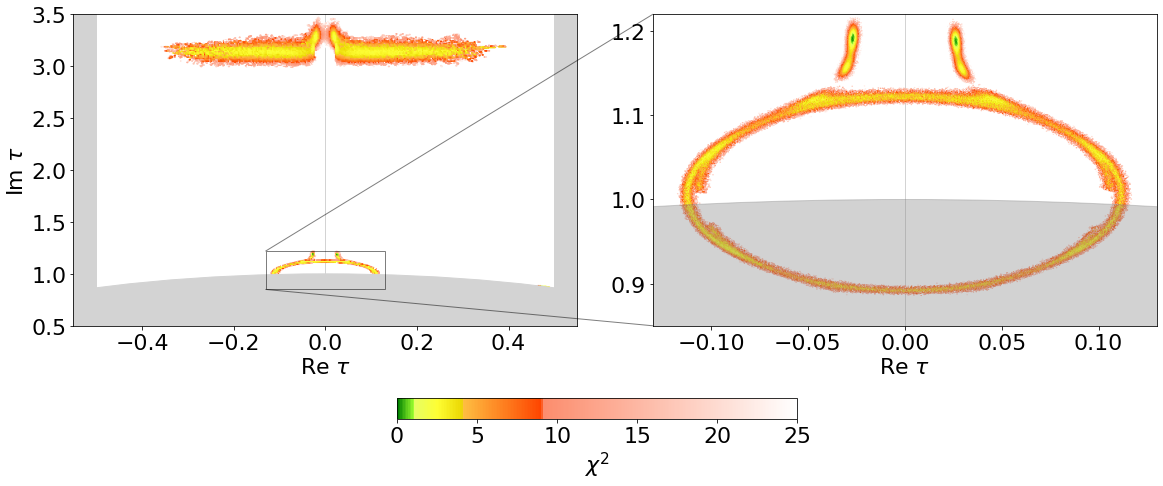
Moduli space

Let us take a look on how the points are distributed over the modulispace, see also figure 2 of the paper

# Some more advanced plots
import matplotlib.pyplot as plt


def RetauImtauplot(df, gridsize=200, cmap='ocean', extent=None, sizefactor=1.5, fontsize=22,
                   colorbar=True, axlines=True,
                   zoom_in=False, zoom_in_loc=[1.15, 0, 1., 1.], zoom_in_extent=[-0.22, 0.22, 2.95, 3.45],
                   zoom_in_gridsize=500):

    plt.rcParams.update({'font.size': fontsize})

    fig, ax = plt.subplots(figsize=(sizefactor*6.18,sizefactor*3.82))

    im = ax.hexbin(df['Retau'], df['Imtau'], C=df['chisq'], reduce_C_function=np.min,
                   gridsize=gridsize, cmap=cmap, extent=extent, vmin=0, vmax=25)
    if not extent==None:
        ax.set(xlim=(extent[0], extent[1]), ylim=(extent[2], extent[3]))
    ax.set_xlabel(r'$\mathrm{Re}~ \tau $');
    ax.set_ylabel(r'$\mathrm{Im}~ \tau $');

    ax.set_aspect(abs((extent[1]-extent[0])/(extent[3]-extent[2]))*(3.82/6.18))

    if axlines==True:
        ax.axvline(0, color='lightgray', lw=1, zorder=0);
        ax.axvline(0.5, color='lightgray', lw=1, zorder=0);
        ax.axvline(-0.5, color='lightgray', lw=1, zorder=0);

        ax.add_patch(plt.Circle((0,0), radius=1, facecolor='lightgray', edgecolor='lightgray'));

        ax.axvspan(0.5,10, facecolor='lightgray');
        ax.axvspan(-0.5,-10, facecolor='lightgray');

    if zoom_in==True:
        axins = ax.inset_axes(zoom_in_loc)
        axins.add_patch(plt.Circle((0,0), radius=1, facecolor='gray', edgecolor='gray', alpha=0.35));
        axins.hexbin(df['Retau'], df['Imtau'], C=df['chisq'], reduce_C_function=np.min,
               gridsize=zoom_in_gridsize, cmap=cmap, extent=zoom_in_extent, vmin=0, vmax=25)
        axins.axvline(0, color='lightgray', lw=1, zorder=0);

        # sub region of the original image
        [x1, x2, y1, y2] = zoom_in_extent
        axins.set_xlim(x1, x2)
        axins.set_ylim(y1, y2)
        axins.set_xlabel(r'$\mathrm{Re}~ \tau$');

        ax.indicate_inset_zoom(axins, edgecolor="black")

        axins.set_aspect(abs((zoom_in_extent[1]-zoom_in_extent[0])/(zoom_in_extent[3]-zoom_in_extent[2]))*(3.82/6.18))

    if colorbar==True:
        cax = fig.add_axes([0.62, -0.1, 0.6, 0.05])
        fig.colorbar(im, cax=cax, orientation='horizontal').set_label(r'$\chi^2$', rotation=0);#, labelpad=10);

plotargs = {'cmap':mf.flavorpy_cmap(),  'gridsize':400,
            'zoom_in':True, 'zoom_in_gridsize':800, 'zoom_in_extent':[-0.13, 0.13, 0.85, 1.22]}
RetauImtauplot(df_mcmc_NO, extent=[-0.55,0.55,0.5,3.5], **plotargs)

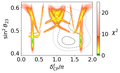
s23^2 - d/pi

Let us try to reproduce the first panel of figure 3 of the paper

ax = mf.plot(df_mcmc_NO, x='d/pi', y='s23^2', show_exp='2dim', gridsize=400, vmin=0, vmax=25);
ax.set_xlim(0, 2);

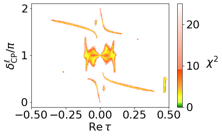
Retau - d/pi

Let us see whether we can reproduce the left panel of figure 5 of the paper:

ax = mf.plot(df_mcmc_NO, x='Retau', y='d/pi', gridsize=400, vmin=0, vmax=25);
ax.set_xlim(-0.5, 0.5);

Inverted Ordering

Moduli space

Let us take a look on how the points are distributed over the modulispace, see also figure 2 of the paper

plotargs = {'cmap':mf.flavorpy_cmap(),  'gridsize':400,
            'zoom_in':True, 'zoom_in_gridsize':300, 'zoom_in_extent':[-0.05, 0.05, 1.48, 1.72]}
RetauImtauplot(df_mcmc_IO, extent=[-0.55,0.55,0.5,3.5], **plotargs)

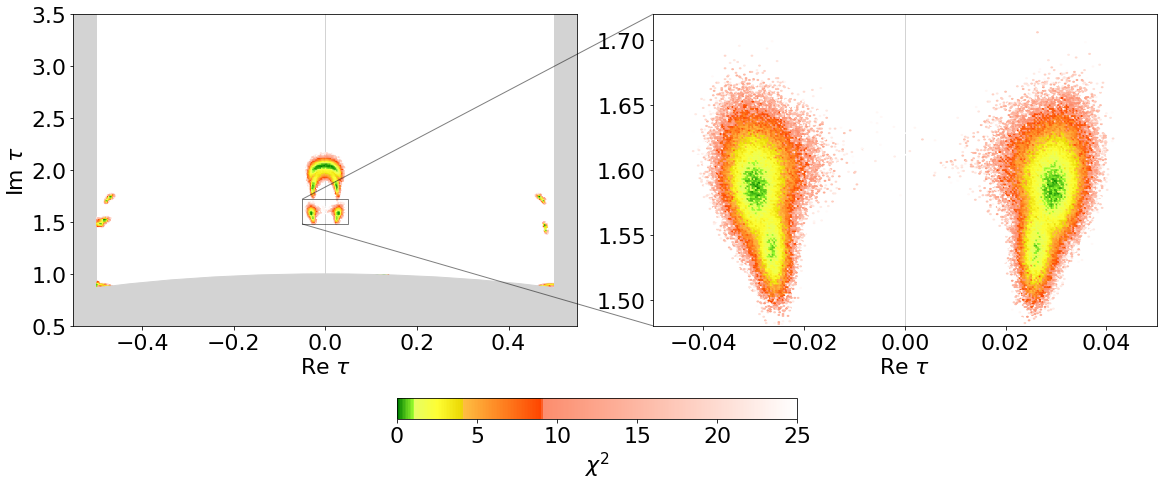
Appart from many additional viable regions, also the shape of the minima reported in the paper look a bit different here due to the more recent experimental data.

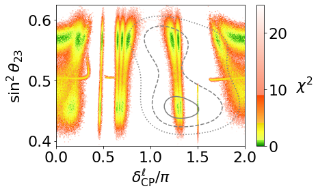
s23^2 - d/pi

Let us try to reproduce the first panel of figure 4 of the paper

ax = mf.plot(df_mcmc_IO, x='d/pi', y='s23^2', show_exp='2dim', gridsize=400, vmin=0, vmax=25);
ax.set_xlim(0, 2);

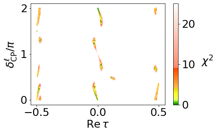
Retau - d/pi

Let us see whether we can reproduce the right panel of figure 5 of the paper:

mf.plot(df_mcmc_IO, x='Retau', y='d/pi', gridsize=300, vmin=0, vmax=25);

Conclusion

We were able to reproduce the results of the Weinberg Operator Model of the paper with around 30 minutes of computation time on a conventional desktop machine. Further investing some 3-4 hours of computation time, we could also find and explore additional experimentally viable regions in the parameterspace of this model.